TUNING NETWORK HYPERPARAMETERS
In machine learning, there are a number of hyperparameters that affect the quality of an algorithm’s predictions. These hyperparameters include the following:
- Number of Epochs
- Batch Size
- Training Optimization Algorithm
- Learning Rate
- Dropout Regularization
- Number of Neurons in Hidden Layer
- Lag Window
The technique I utilized for optimizing my hyperparameters was a grid search. A grid search is a brute force method that can be applied across all machine learning models. Grid-searching builds on each possible combination of model parameters and stores a model for each. Once all of these models are built, their performance can be evaluated, and the optimal parameters selected for the final model. The following sub-sections will discuss the results of this hyperparameters search and explain the choice for the final algorithm design.
1. Number of Epochs and Batch Size
The number of epochs denotes the amount of times the entire set of input training data is passed through the neural network during training. It is necessary t utilize multiple epochs during training because this allows the network to change its weights during training. Using too few or too many epochs can cause the network to underfit or overfit; both of these scenarios cause the network to have poor performance. Basically, supervised machine learning attempts to approximate a target function that maps its given historical inputs to historical outputs. Because a function is being approximated, the function should just be a generalization as we only have an incomplete, noisy sample of data. This generalized function is referred to as inductive learning, meaning the machine learning algorithm is trying to learn general concepts that are underlying in the specific training data. This idea of generalized learning is important because it allows a machine learning algorithm to use these general concepts to make predictions on future data. In order for the algorithm to learn generalized concepts, we want to avoid overfitting, which means that the algorithm is too well trained on the training data. Overfitting means that the model has learned too much detail about the training data (such as noise), so the model will be unable to generalize. As a result, the model will not be able to make accurate predictions on unseen data. Conversely, underfitting means that the model does not account for the underlying relationships in the given data, which also will result in poor model performance. The goal for selecting the number of epochs is avoiding overfitting and underfitting to optimize model performanceThe grid search was performed on ten stocks from the IT sector. The table below shows a sample of the experiments that were run. In the set of experiments shown in Table 6 below, the batch size was kept constant at size 50, and the number of epochs were varied. The best results were achieved using 10 epochs. (It should be noted that this also had a lag window of 1 and uses the Adam optimizer). Representative results of the extensive testing for day-ahead forecasts for IT sector stocks are shown in Table 6 below.
Table 6: Testing Number of Epochs for LSTM
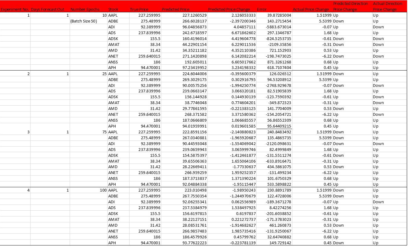
The results showed that training using 10 epochs and 50 batches yielded about 70% in predicting the direction of next-day stock movements, though these day-to-day predictions still show a high degree of error. As the number of epochs increased, the prediction error for the direction that stocks would move quickly increased. An examination of the data as it trains over a number of epochs (as shown in Fig. 19) reveals that the accuracy quickly increases the model trains, and then levels off over time despite the increasing number of epochs.
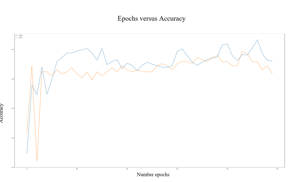
Fig. 19: Number of Epochs versus Accuracy of the LSTM. Note that the orange line denotes the test data, while the blue line denotes the training data.
2. Optimization Algorithm
The optimization algorithm is an important part of training a machine learning algorithm that works in tandem with the loss function. While an algorithm trains, the weights and biases of the network are changed, affecting how well the model models a given dataset. The output of the loss function is high if the network predictions based on the model are poor. Conversely, better predictions mean the loss function output is lower. A model’s optimizer bridges the gap between updating a model’s parameters and the loss function. The optimizer works by tuning parameters and molding the model based on the most accurate assignment of weight values. The optimizer uses the loss function as an indication of the quality of this tuning. The optimizer’s goal is to minimize the loss function. Keras provides a number of optimization algorithms, which can affect the performance of the overall mode. Thus, testing was conducted for the selection of the best optimization algorithm. The different algorithms tested are discussed in the following sections below. Please also note that some sample results from our IT sector stocks are also provided in Table 7. below to give a representation of the testing results.
Table 7.: Sample Testing of Optimizers on IT Sector Stocks

- Stochastic Gradient Descent
Stochastic gradient descent is a gradient-based optimizer. In gradient descent, the effects of small changes in the individual weights in the network on the loss function output are calculated. After performing these calculations, the network’s weight can be adjusted according to the gradient, meaning the algorithm will adjust in a small step in the direction calculated. These two steps are, then, calculated iteratively. The class technique of gradient descent uses all input training samples on every pass to tune a network’s parameters. Instead, SGD uses only a subset of the training samples on each pass. In our results, SGD yielded correct directional estimates of stock movements in about 55-60% of stock price predictions.
- RMSprop
RMSprop is derived from the Adagrad optimizer. While the original Adagrad optimizer allows all of the gradients to accumulate to create momentum, RMSprop creates windows where gradients are accumulated. In our results, RMSprop yielded correct directional estimates of stock movements in about 55-60% of stock price predictions.
- Adam
The Adam optimizer is a gradient-based optimizer. Adam stands for adaptive moment estimation, denoting its use of past gradients to calculate current gradients. Another important aspect of the ADAM optimizer is the use of momentum, wherein fractions of previous gradients are added to current gradients. Momentum is a method that helps accelerate SGD in the relevant direction. More specific details of these results will not be discussed here as this was the default optimizer utilized in the other hyperparameter experiments. (This was done because the Adam optimizer showed the greater performance amongst those tested). . In our results, SGD yielded correct directional estimates of stock movements in about 65-70% of stock price predictions. Because of its edge over RMSprop and SGD, the Adam optimizer was selected for the final design.
3. Learning Rate
Like the loss function, the learning rate is another parameter that is tied to the optimization function. The learning rate regulates how fast the optimization algorithm “learns,” i.e., tunes the weights of the networks. Changing a network’s weights too quickly can mean that the algorithm is taking steps that may be too large that will inhibit the minimization of the loss function. The learning rate is a number that is multiplied by the gradients in order to scale them, ensuring that changes in the weights are smaller. Smaller weights means the algorithm is taking smaller steps, which may prevent the optimizer from stepping over the absolute minimum. The default learning rate for the Adam optimizer is 0.001. Thus, I experimented with increasing the learning rate to see how this affected the accuracy of the predictions. Overall, increasing the learning rate resulted in a quick decrease in the accuracy of the algorithm’s predictions. Some of this sample data is shown below in Table 8. For instance, increasing the learning rate resulted in the algorithm being able to predict the accuracy of price directional movement at about 60%, which represents in a reduction in our previous predictive accuracy. This trend of increasing the learning rate resulted in further reductions continued with further testing, so the learning rate remained set at the default.

4. Dropout Regularization
Dropout is a technique that selectively chooses neurons to ignore (“drop-out”) during training. On a given pass through the network, the contribution of these dropped neurons to activating downstream neurons is removed, meaning their weights are not applied. The motivation underlying dropout is that as a neural network trains, the weights of the neurons settle into their context of the neurons, and neighboring neurons can become too specialized, resulting in a model that is overfit to training data. When dropout techniques are used, other neurons in the network will have to step in to interpret the representation required to make predictions for the missing neurons. It is theorized that this results in the network learning multiple internal independent representations. In Keras, dropout is implemented through the selection of a probability value that randomly selects nodes to be dropped out. The default value of dropout in all of the previous experiments was 0, meaning dropout was nonexistent. As expected, the introduction of dropout produced a severe reduction in the algorithm’s capability to predict price movements. This outcome was expected because dropout interferes with the algorithm’s “memory” capabilities. Thus, no dropout was utilized in the final design.
5. Number of Units.
The number of units represents the number of neurons of a layer. A unit takes inputs from all the nodes in the layer below, does its calculations, and then outputs them to the layer above. Thus, the number of neurons in a layer controls the representational capacity of the network.
Table 9: Testing Effects of Different Numbers of Neurons on LSTM Predictions
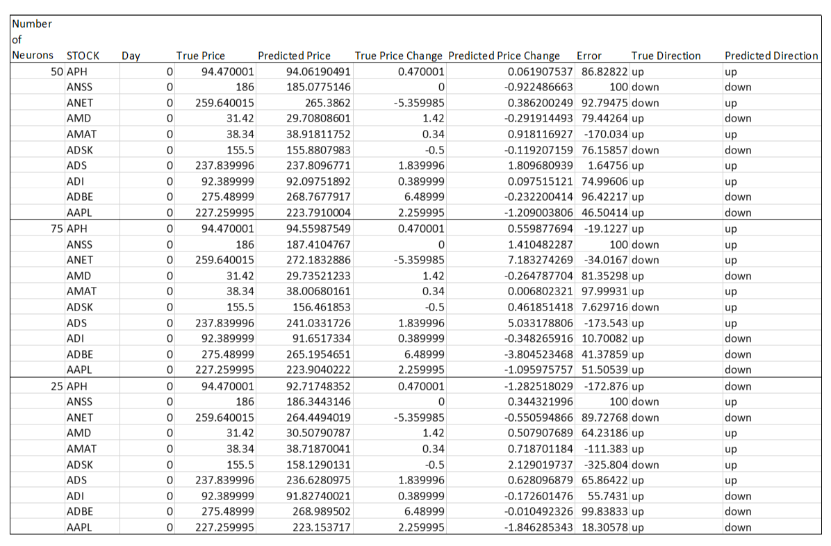
Because 50 neurons have been the default in this testing process, I decided to test number of neurons above and below this number to see if there were any improvements in predictions. The configuration using 50 neurons still had a slight edge in predictive accuracy. Decreasing the number of neurons caused a severe decrease in the ability of the algorithm to predict the correct directional movement of the price, and an increase in the number of neurons still slightly underperformed the 50-neuron configuration.
6. Lag Window
One of the methods tested to counteract concept drift was the idea of a “lag” window. These experiments have been conducted with a window size of one, so increased window sizes were tested to see if they would increase predictive accuracy. Some sample results are shown in Table 10 below.
Table 10: Sample Test Results of Varying “Lag Window”

Overall, the results in the table and other testing showed that a lag window did not increase predictive accuracy. In fact, the lag window caused a substantial increase in error. The addition of a lag window seemed to hamper the algorithm’s ability to make detect directional changes in price movement, which is a highly detrimental result in stock trading.
FINAL DESIGN:
In general, based on the results of hyperparameter testing that are discussed in the sections about the following final design was chosen. The network trains with 10 epochs and a batch size of 50. It contains 50 neurons. Additionally, its optimizer is set to be the Adam optimizer with a learning rate of 0.001. No dropout and no lag window are used.