A two-dimensional visual motion detector based on biological principles
Adam Pallus and Leo J. Fleishman, Department of Biological Sciences and Center for Bioengineering and Computational Biology, Union College, Schenectady, NY 12309, USA.
This report describes a biologically-inspired computer model of visual motion detection. The model is designed to use sequential digital frames (e.g. typically from digital video of natural scenes) and detect the local direction and relative strength of motion in any portion of the scene. The aim of creating this model was to study the ways that changes in the properties of simple motion detection circuits alter the way in which natural moving stimuli are likely to be perceived. The model is based on a 2-dimensional grid of “correlation-type” motion detector, frequently referred to as “Reichardt detectors.”
A review of this type of motion detection can be found in Borst and Egelhaaf (1989). The idea of analyzing two dimensional scenes with a grid of simple motion detection circuits comes from the work of Johannes Zanker (e.g. Zanker 1996; 2004).
Credits
We were originally introduced to the idea of using this type of motion-detection modeling to analyze natural scenes by Jochen Zeil of the Australian National University in Canberra. Our model is based directly on that described by Johannes Zanker (Zanker 2004; Zanker and Zeil 2005), who graciously provided a working version of his model as well advice concerning its implementation. The version of the model presented here is written by us in MATLAB, but it is based directly on Zanker’s model. Anyone choosing to use the programs presented here in published work should cite Zanker (1996). The work presented here is the result of a joint effort by Adam Pallus, Leo Fleishman, Michael Rudko and Laura DeMar of Union College and was supported by a grant from the Howard Hughes Medical Institute to Union College.
The model
This model consists of a two-dimensional grid of elementary motion detection circuits (described below). Each of these circuits obeys simple processing rules, and yet the program is surprisingly effective at detecting and quantifying motion even in very complex scenes. The mathematical underpinnings of the model are described in Zanker (1996). We have implemented Zanker’s model using MATLAB programs. The elementary motion detection units of the model are correlation detectors (often referred to as “Reichardt detectors”). They function by comparing the spatial distribution in light intensity of scenes displaced in time. Correlated shifts in time and space are interpreted as motion.
Here we first give an example of how the motion detector program works. In section II we describe the theory underlying how it works. Section III provides a series of examples of different scenes analyzed using the motion detection program. In section IV we illustrate an attempt to address a specific question: can a motion detector circuit be tuned so that it acts as a filter allowing a visual system to tend to ignore motion of windblown vegetation while being responsive to animal motion? Section V includes the programs that allow a user with access to the MATLAB programming language (and the Graphical Analysis Toolbox) to run the programs themselves along with a manual for their use, as well as a description of the underlying logic.
An example of the motion detection program
The following two examples are .GIF animated files. In each example the first video shows a natural scene filmed with a digital video camera. The second and third clip show the output of the motion detector presented in two ways. In the first scheme, motion direction is shown with color and the strength of motion detector output (in arbitrary units) is shown by the intensity of the color. In the second scheme motion direction is not preserved, and the strength of motion detection output is shown as a three dimensional graph.
Click to view the animated examples.
Motion detection models in general
A. General importance of visual motion detection.
A critically important feature of nearly all animal visual systems is the detection and analysis of motion. Retinal motion can be produced both by movements of the animal’s eye and by the world around it. To make use of the information the animal must be able to distinguish the classes of motion and in many cases make corrective eye or head movements to minimize certain classes of motion. When an animal and/or its eyes are in motion the distribution of local movement direction and velocity at different locations on the retina can tell the animal a great deal about properties such as the shape and distance of different objects and the nature of the animal’s own movements. Equally important, detection and analysis of movement of objects in the outside world can be tell an animal that food, predators, or members of its species are present. In order to acquire such information the animal must be able to distinguish important motion from unimportant motion such as that of windblown vegetation. If one wants to convince oneself of the important role of motion in finding living objects in the natural world one merely has to go into a forest and go bird-watching. Invariably it is the abrupt movement of leaves or branches which reveal the presence of a bird (or other animal). Moreover such motion is fairly easy to detect even if a moderate breeze is causing considerable motion of the surrounding vegetation. You can imagine how much more important motion perception must be to an animal which either eats living prey, or is itself the potential prey of larger animals whose approach is often revealed by movement.
B. Attention and movement
Many animals have a retina which consists of a broad area of visual field which is of moderate or low visual acuity, and a smaller, usually centrally located, area of high visual acuity known as the fovea. Typically central attention within the brain is directed to the small part of the image of the world that sits on, or near, the fovea. Thus the retina scans a broad area of visual space and when something of potential interest or importance is detected in the visual periphery its image is brought onto the fovea with a reflex shift of the position of the eye. This reflex is known as the “visual grasp reflex.” The combination of a broad retinal field of view and a reflex which brings the gaze onto important portions of it serves as an efficient way to process a large amount of visual information. The nervous system must have a fast and fairly simple scheme for “deciding” when to shift gaze toward a new location. The strongest stimulus for the visual grasp reflex is motion in the visual periphery. This makes sense for most animals because potential prey moves, potential predators move and potential mates or competitors move. This movement in the visual periphery often indicates the presence of a potentially important cue. However, as mentioned above, the world is also full of irrelevant motion. For terrestrial animals this is mainly in the form of windblown vegetation while for aquatic animals this is in the form of wave action. Thus, in addition to responding to motion an attention-system must have some way to filter relevant from irrelevant motion.
C. Modeling motion detection at the neural level
One might suppose that in order to detect a moving object a visual system would first have to identify an object at two different moments in time and note that its position had shifted. However such a sensory task would be quite challenging and presumably fairly slow. It has been shown both with computer models and studies of visually sensitive neurons in a wide variety of animals that it is not, in fact, necessary to identify objects in a visual scene in order to detect local motion. Over the last several decades several models have been put forward that suggest that it is possible to detect the location, direction, and possibly the velocity of motion on small patches of the retina without any higher visual analysis. One would expect such a simple localized motion detection scheme to underlie a process such as the visual grasp reflex. One would also imagine such a process would underlie the determination of localized optical flow (i.e. local estimates of motion direction at different retinal locations induced by self-motion). The point is that there are many cases where it is important to quickly and simply recognize the presence of motion without taking the time or neural complexity required to track objects in a visual scene.
A variety of models of the neural basis of motion detection have been proposed. One model that has received a great deal of attention is known as a “correlation-detector.” While this type of model is not the only one that has been identified as important, it has been shown in a number of different species (including, for example insects and humans) that the early stages of motion processing seem to be controlled by an algorithm similar to that presented here: namely a correlation detector.
D. The basic design of a correlation detector
A correlation detector is a simple neural network that extracts a directional motion signal from a series of sequential frames of a visual scene. The basic design of the circuit is shown in Figure 1.
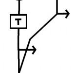
Figure 1. The basic design of a correlation detector.
In its simplest form it consists of two detectors of light intensity (e.g. two receptive fields on a retina) which are spatially separated. The output from each detector is a signal equal to (or proportional) to the intensity of the light falling on it. The outputs from the two intensity detectors are multiplied together to give the motion detector output. However the lines carrying the signal from intensity detectors to the multiplier differ. The line from the first intensity detector delays and spreads out the signal by acting as a low pass filter. The basic operation is illustrated in figure 2a-c. If the stimulus is moving in the correct direction at approximately the correct velocity the two signals superimpose and give a strong output. If the moving stimulus is going in the wrong direction, or if the timing does not match the circuit properties well a small signal, or no signal is produced. This simple circuit responds to motion in one direction. The response is also velocity tuned.
Click to view the full size animations.
Figure 2. These three animations illustrate how a correlation detector functions. Note that there is strong output only when the direction and timing of the motion are matched to the properties of the detection circuit.
The model circuit has two basic parameters that can be manipulated: the spacing between the two detectors (= S), and the low-pass filter properties of the delay line. The behavior of the delay line is determined by a time constant (T). Large values of T result in a slower, more spread out response, while small values of T yield a very rapid response. If the spacing, S, is kept constant large values of T make the circuit responsive to relatively slow motion, while short values of T make the circuit sensitive to rapid motion. T is defined in units of frames of input.
It is also worth noting that the response of the motion detector depends on the intensity of the moving stimulus. This is a somewhat troublesome confounding effect. Later we will explain various steps that reduce the impact of this effect, but ultimately the sensitivity of the correlation detector to contrast (i.e. the intensity of the moving stimulus relative to the stationary background) is a limiting feature of the model.
E. Additional aspects of the correlation detector model.
(1) Subtraction step
The model as presented above is simplified. Some other steps are required to make such a model behave in biologically realistic manner. First of all the model as presented will give different strength outputs based simply on spatial correlations in brightness of different locations in the absence of motion. For example if a bright stripe sits over both detectors, even without motion their outputs will be high and then multiplied together. In order to make this circuit a MOTION detector another step is required which is illustrated in Figure 3.
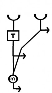
Figure 3. The elementary motion detector (EMD) consists of two correlation detectors connected in a reciprocal fashion. The output from from the two detectors is then subtracted.
The detector circuit has to perform the basic steps shown above in two directions, and the outputs from the two detectors are subtracted. This step eliminates any output that stays the same across time. Only outputs resulting from frame to frame change result. Additionally any output resulting from spatially uniform changes in lighting (e.g. flickering light) are eliminated by the subtraction step.
Notice that the final output of this more complete detector is still directionally sensitive, with the sign of the output giving the predominate direction of motion.
(2) Spatial filtering of the input image
As described in more detail below, our motion detection model is built up of a 2-dimensional array of detectors like that shown in figure 2. The input for our model is sequential frames of video. However in order to make analysis of these scenes biologically realistic we need to carry out some processing steps that occur in animal visual systems. In our model we assume that light is detected by some type of cell (e.g. retinal ganglion cell) with a center-surround type visual field. All of the receptive fields have an excitatory center and an inhibitory surround. This type of interaction can be well modeled as the difference of two Gaussian (i.e. normal) distributions: a narrower positive Gaussian and a broader negative Gaussian (Wandell 1995).
Here we imagine that each scene is viewed by an overlapping array of these visual fields. In practice this is implemented by filtering each frame with a difference of Gaussians (DoG) spatial filter. The filtering process makes each point the average of many surrounding points. First the positive Gaussian is determined, then the broader negative Gaussian and the second is subtracted from the first. This is carried out for every point in the scene. The process and an example of its application are illustrated in Figure. 4 and 5.
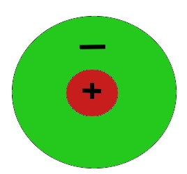
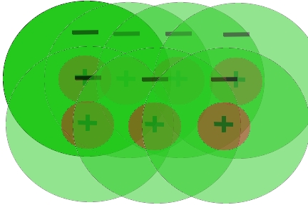
Figure 4. A. Inputs to the model are on-center off-surround receptive fields like that shown here. B. Since the model takes input from every pixel, the input to the model can be thought of as consisting of a set of overlapping receptive fields. C. The center-surround field is create by having each point be the weighted average of the points surrounding it. The weightings take the form of two Gaussian distributions of equal area. The broader Gaussian is subtracted from the narrower one. This type of filtering is referred to as a Difference of Gaussian, or DoG filter. D. The resulting filter shape after subtracting the broader “inhibitory” Gaussian distribution from the narrower “excitatory” Gaussian.

Click the images to view them full sized.
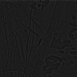
Figure 5. Two stationary scenes. The first as originally recorded. The second after DoG filtering has been applied to every pixel. Note the DoG filter enhances edges while making the average intensity of the scene = 0.
There are two main effects of the DoG spatial filtering: (1) the average intensity of the scene goes to zero which makes the model insensitive to the overall brightness in a scene, and (2) edges are strongly enhanced. This is precisely what the center-surround receptive fields of animal visual systems accomplish.
This spatial filtering is a critical step in our motion detection model, and it is worth taking a moment to consider what the effects are of changing the spatial properties of the filter. In the model we allow the user to select the shape of the Gaussian filters by choosing the standard deviation as shown above (Fig. 4). In general we make the negative Gaussian twice the size of the positive Gaussian. The width of the negative Gaussian is essentially defining the size of the receptive field of the inputs to the motion detector. It determines the spatial frequency resolution of the detector. In order to avoid aliasing the width of the receptive field should be twice the spacing (S) between detectors. Aliasing is simply the case where the motion detector circuit is stimulated over time, not by the same moving edge, but by different portions of the scene that happen to move over it. By matching the receptive field to the spacing of the inputs, this cannot occur. Thus the size of the receptive field and the spacing of the motion detection inputs are closely linked. In fact, in biological systems, this also occurs.
F. The 2dmd model
The next step in implementing our model is to program the interactions described above into a two dimensional grid. The program starts with a sequence of video frames. After adjusting the dimensions of the input video, the video is (a) converted to grayscale and (b) filtered with the appropriate (DoG) filtering. The motion detector asks for spacing s in terms of number of pixels between adjacent detectors. Each pair of pixels to the right and to the left and up and down are interconnected to form the array of paired elementary motion detectors.

Figure 6. This figure is reprinted from Zanker (2004). It illustrates the basic steps in our model. A video sequence is analyzed. First every frame is converted to gray scale. Then each frame is spatially filtered. Then they are processed through the two dimensional motion detector as shown.
The next input parameter is the time constant T for the delay step. The basic computational algorithm starts with creating a temporally filtered version of the entire video sequence. This is done by passing the sequence of frames through a low pass temporal filter with the chosen time constant. For each frame of video motion detection output is determined at every pixel. The motion detection output is the intensity of the pixel in the frame that is not temporally filtered, multiplied by a point shifted in space by s pixels on the temporally filtered version of the video. This is done in each pair of directions and the results subtracted. This entire process is done for the right left pairs and the up-down pairs. For each point this gives us a y-value (up and down) and an x value (right-left). The direction of motion is cosine(y/x) and the magnitude of direction is (x2+y2)0.5. The output for each frame and each pixel is then plotted either as a color graph (color = direction, intensity = output strength) and a three dimensional graph of output intensity.
G. Model parameters
Adjustable parameters in the model are the “width” of the Gaussians in the DoG spatial filter (the width of ± 1 standard deviation of the mean), the spacing parameter (S), and the time constant of the low pass filter (T).
H. Model output
The output of the model is a value for pixel in each frame of video (starting a few frames after the first). The intensity of the output is simply the output strength from the motion detector at that location – it has no real units. We provide two ways to plot the motion detector output. We can plot it using color, where the intensity of the point indicates the magnitude of the output, and the color indicates the direction as shown in Figure 6. We can also ignore the directional information and simply plot the strength of motion output at each location in a three-dimensional graph.
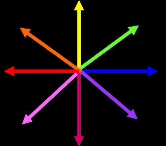
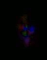
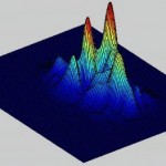
Figure 6. A. In the color plots the primary direction of motion is indicated by the color, according the directions shown in this graph. Strength of output of the detector is given by the intensity of the color. B. An example of a frame of motion detector output in color. C. A second way of plotting the motion detector output is to show the output strength vs. position with a 3d graph. This plot gives no information about the motion direction.
EXAMPLES OF MOTION DETECTION ANALYSIS
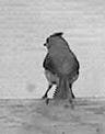
The following give examples from three types of motion. We show a cricket running, a bird jumping, and vegetation blowing in the breeze. For each example we illustrate the effects of changing the time constant, T and space constant S. In all cases the DoG filter parameters are set so that the input the standard deviation of the wider (i.e. negative) Gaussian filter is twice the spacing parameter S.
Figure 7. Bird Jumping Cricket Running Vegetation Blowing
A PROBLEM IN MOTION DETECTION
Suppose you are a small animal living in dense vegetation. In our lab, for example, we work on small arboreal lizards. Your world is surrounded by motion. Motion of animals (e.g. prey, potential predators, conspecifics) is very important and you should generally direct attention toward such movements. However, there is lots of blowing vegetation which creates a constant source of irrelevant motion or noise. How does the sensory system filter out relevant from irrelevant motion? One possibility might be to carry out filtering at the very beginning of the motion detection process.
Here we ask, can the motion detection grid be made more responsive to animal motion and less responsive to vegetation movement simply by changing the input parameters?
The examples in the previous section suggest at least a partial solution. As can be seen, larger time constants (i.e. slower response time and longer delay) give stronger outputs overall for vegetation. The smaller time constants (fast response) tend to give higher values for faster movements. This suggests that an attention system with low values of the delay time constant T, will tend to be more responsive to animal, than to plant motion.
Finally we present of a lizard sitting in dense vegetation that is moving in the breeze. The lizard performs a “push-up” display. We run this scene through the motion detection model with two different values of the time constant T.
Figure 8. Analysis of a lizard giving a visual display in its natural habitat.
Note that with a short time constant (T), the lizard is much more visible than the vegetation.
This suggests that motion detector tuning can be used, at least in part, to filter out irrelevant from relevant motion. We are currently studying this problem more carefully to see if this process can actually be demonstrated in living animals.