Train, validate and test partitions for out-of-time performance take planning and thought
(This piece is also at TDS.) The purpose of supervised machine learning is to classify unlabeled data. We want algorithms to tell us whether a borrower will default, a customer make a purchase, an image contains a cat, dog, malignant tumor or a benign polyp. The algorithms “learn” how to make these classifications using labeled data, i.e. data where we know whether the borrower actually defaulted, customer made a purchase, and what a blob of pixels actually shows. Normally, researchers take the labeled data, and split it three ways: training, validation and testing/hold-out (the terminology sometimes differs). They train hundreds of models on train data, and select one model that performs well on the validation data. The reason for using only a subset of labeled data to train the algorithm is to make sure that the algorithms perform well on any data – not just the data used to train the algorithm. Researchers often repeat this step several times, selecting different splits into train and validation, making sure the model performance is not specific to a particular validation data (k-fold cross-validation). As a final step, researchers evaluate the model’s performance on yet unseen data (the test set). This provides a measure of how well the model will perform on the unlabeled data. This classic setup is illustrated in the figure below:
 Figure 1: Classic train, validate and test split
Select model that performs well on ‘validate’
Evaluate its performance on ‘test’
.
In a large number of applications the data has a time dimension such that the labeled data is the past and the unlabeled data is the future. For example, we already know which borrowers or customers defaulted or made a purchase in the past. We want to know which ones will do so in the future. In this case, the purpose of the algorithm is to
predict labels ahead of time. This means that it needs to work not just on yesterday’s data but also on tomorrow’s. I ask how the time dimension should be incorporated into the classic train/validate/test setup. This will surely matter if the processes that change over time. It turns out that there is a whole
sub-field dealing with this issues. The approaches range from setting up a sliding window over training data, to actively testing for a changes in the underlying relationships. In this post, I review a few options for setting up the train, validation and test data.
Option 1: in-time validate, in-time test
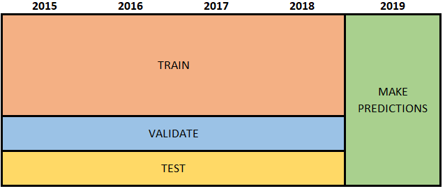
Let’s consider what happens if we ignore the time dimension of the data, and split all of the labeled data regardless of its time dimension. We train, validate and test the model using data from the same time period. We make predictions for new data (say 2019) using using a model trained, validated and tested on labeled 2015-2018 data. The figure below illustrates this set up. The advantage is that we use the most recent data to train the model. The disadvantage is that it assumes that the relationships that existed in the past will be the same in the future. If the relationships shift over time, our estimated performance measures (which we calculated using in-time test data) will overstate the model’s true performance, i.e. once deployed, the model will perform worse than we expect.
Option 2: in-time validate, out-of-time test
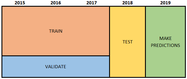
Another possibility is that we hold-out year 2018, train the model using 2015-2017 data, and test it on 2018 data. The advantage of this approach is that we explicitly evaluate the model’s ability to predict out-of-time. The disadvantage is the ability to predict out-of-time is not taken into account when building the model. This is because we select model that performs well on the in-time validation data. Moreover, unless we re-train the model using the full 2015-2018 data, we are not using the most recent data to make predictions.
Option 3: “walk-forward”
Roger Stein suggests training models on successive (potentially sliding) windows of data, and making predictions for the next time period. Each time we retrain the model using all observations through a particular point in time, and make predictions for the next time period. The predictions from each window are combined into one set of predictions. We do this for many different models and choose one that creates best combined predictions. The advantage of this approach is that the model building (i.e. trying out which models work best) explicitly takes into account the model’s ability to make out-of-time predictions. Since the model is refit for each window, this approach simulates periodic retraining of the model which happens (or should happen) in practice. The disadvantage of the approach is that we always validate predictions on the same set of data rather than randomly selected data. (Perhaps holding out a portion of the test data could overcome this concern.)
To retrain or not to retrain
When we make predictions into the future, it is probably a good idea to use as recent data as possible so that we capture the most recent phenomena. However, if we hold out the most recent data (to evaluate out-of-time performance) as in option 2, we should probably re-train the model using all of the labeled data before making predictions. The retraining is illustrated in the figure below:
.
There is some
disagreement online over whether to re-train the model using all training and test data before deployment.
Kuhn and Johnson seem pretty explicit when in chapter on over-fitting, data splitting and model tuning, they say “We then build a final model with all of the training data using the selected tuning parameters.” (page 65). Similarly, Andrew Ng in one of his
lecture notes says that after selecting a model from a cross-validation procedure we can “optionally” retrain the model “on the entire training set.”
.
It is helpful to draw the
distinction between model parameters and hyper-parameters (aka tuning parameters). Hyper-parameters determine the
structure of the model and generally can’t be estimated from the data. They include things like the tree complexity, k in the KNN algorithm, feature set, functional form (e.g. linear vs quadratic) etc. In contrast, model parameters include coefficients in a regression, tree rules, support vectors. These can be estimated using data. The model building stage is all about finding the hyper-parameters. Once, the hyper-parameters (i.e. the structure of the model) are validated, there seem little reason not to use as much data as possible to get the most accurate estimates of the model parameters. These parameters should be used to deploy the model and make classifications or predictions.
Conclusion
In summary, if we follow the classic setup and ignore the time dimension of our data as in option 1, we have no idea how the model will do on out-of-time data. In option 2, we at least have a measure of the model’s out-of-time performance. However, it is only if we do something like in option 3 that we are building models with the intent to forecast the future. Regardless of what we do, retraining the model using all labeled data before making predictions seems like a good idea.
.
I am hard-pressed finding examples of applications that don’t have a time dimension. I suppose a pile of MRI images of which only some were labeled is one example, but my sense is that these one-off projects are rare. Moreover, while some processes are stable over time (e.g. weather or image classification – dog today will look the same as a dog tomorrow), processes such as customer behavior are bound to change over time. It is therefore surprising that the discussions (and implementation) of out-of-time testing and validation are not more ubiquitous. Chances are that out-of-time performance is worse than in-time, particularly if you have lots of in-time labeled data, not a very long time series, and a non-stationary process. However, not doing some out-of-time evaluation could haunt developers as subsequent data will show that the model performed worse than the in-time performance measures indicated.

 Figure 1: Classic train, validate and test split
 Figure 4: “walk-forward” approach, out-of-time validate
 Figure 2: in-time validate and in-time test
 Figure 3: in-time validate, out-of-time test
 Figure 5: once hyper-parameters are set, re-train the model using all labeled data