We have licenses for several data analysis software packages, including basic peak search, peak matching with phase databases, Reitveld refinement, and small angle scattering (SAXS). This page introduces basic peak searching and matching. The help files are generally excellent, and include step-by-step procedures in many cases, so check them out.
Search peaks direct from the pattern
Basic peak search
Peak labeling on pattern
Phase identification
Advanced data analysis
Search peaks direct from the pattern

First, you can access pattern manipulations direct from the XRD Measurement tab. Right-click on the pattern window, and follow the menu tree.
Basic peak search
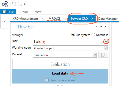
Click on the Powder XRD tab. From this tab you can access peak searching, peak matching, width profiling, background modeling, Reitveld refinement, and other things. In the Flow bar, under Task:, pick Basic, and click the Load data button.
Note that all small angle X-ray scattering data analysis is done via the MRSAXS tab.
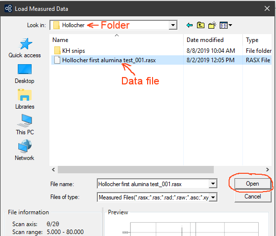
Navigate to your data folder, select the data file you want, and press Open. The file should open, the pattern is displayed in a window, and the peaks are found and listed using the default peak search parameters.
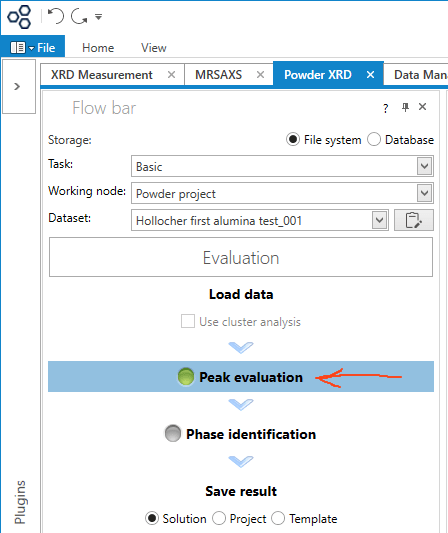
In the Flow bar, click the Peak evaluation button.

Usually, the loaded data file will open with the pattern (Peak Profile View tab), though it may open with a table of detected peaks (Peak List tab).
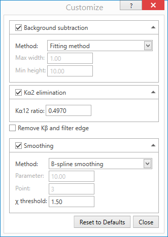
To the right is the Peak Profiling window, where peak detection parameters can be set.

If you are not already there, pick the Peak List tab, from the tab row at the bottom. The Peak Profiling window, shown here, is sometimes invisible to the right. change window widths to bring it back if you can’t see it.
Click the Search and replace peak list radio button, to refresh the peak list each time the Run button is pressed.
In the Peak Profiling window you can select a number of different variables in the peak search algorithm, including pattern modeling method, method to find the peak positions, and statistical variables. Press the Run button to apply changes.
Most important, different choices can reduce or increase the number of identified peaks, allowing you to set a threshold between what is noise and what is an identified peak. For example, try changing the σ cut: value, and watch the number of detected peaks change. Values for σ cut of 10 or more are not unusual.
The Peak List can be exported as a .CSV file, for spreadsheet reading, using the export button to the upper-right of the peak list table.
Labeling peaks
Back to the Peak Profile View tab. Here, the detected peaks are all numbered, but wouldn’t it be nice if the d-spacings or 2Θ angles could be shown, too?
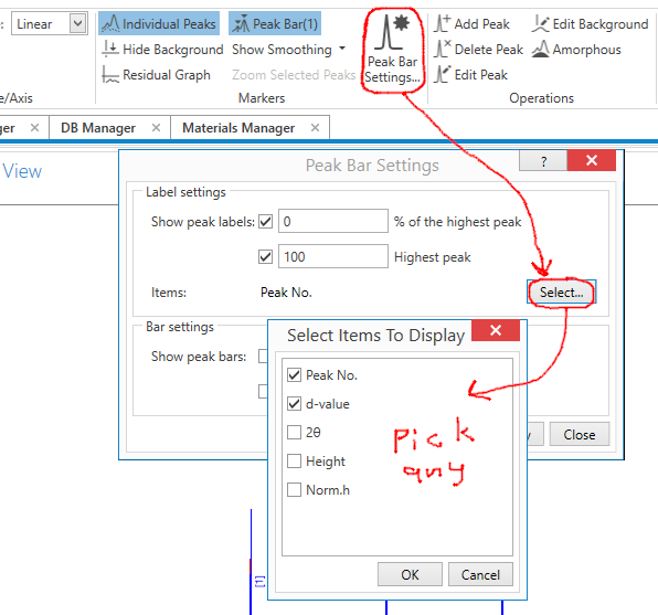
In the menu bar above, pick Peak Bar Settings, press the Select button, then check each thing you want labeled on the peaks. I should warn you that more than two things are likely to run off the graph, and can really start crowning things.
By the way: Individual Peaks, Hide Background, and other settings to the left of Peak Bar Settings will turn on and off different parts of the XRD pattern display.

Here you can see that the peaks now have both the peak number, keyed to the Peak List, and also the d-spacing values, with uncertainties in the last places.
This pattern can be exported either as an image file (you pick the resolution first), several types available, or as a data file, probably .CSV, which presumably has data for each 2Θ increment.
Phase identification

Click the Phase identification button.

The Phase Identification window opens. Press the Search/Match button to start.

This shows the Search/Match window, Subfile tab. There are an awful lot of files in the databases (includes JCPDF and NIST, among others). It’s best to pick one or a few pertinent databases rather than to use all of them. Using too many databases gives you a huge list of results to wade through, almost none of which have any relevance to your sample.

This shows the Search/Match window, Elements Filter tab. There are also an awful lot of elements to make phases out of. It’s best to start by eliminating all elements, then adding the possible or probable ones. Clicking the big, color coded Unknown, Not Included, Included, and Include One At Least buttons changes the color and category of all elements. Repeatedly clicking on one element cycles through the color categories for that element. Repeatedly clicking the arrow next to a row or column cycles through the color categories for that row or column.
It’s stupid to waste time on phases containing elements that are impossible in your sample. Pro tip based on true stories: don’t forget hydrogen and oxygen in samples that may contain water or OH groups.
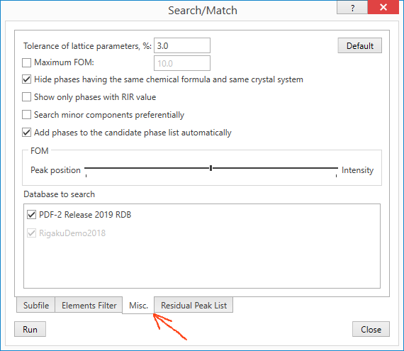
This shows the Search/Match window, Residual Peak List tab. It’s a list of all peaks found, but allows you to restrict the ones used for searching and matching by selecting manually, and/or selecting only peaks with greater than a certain probability of being a real peak (Select I>(e.s.d.) = Select only peaks with peak probabilities greater than X standard deviations).
Once you are happy with the database search criteria in all four tabs, press Run.

When the search/match procedure is done, you are given a list of the possible matching phases. Remember that the lower the figure of merit, the better the match. Think of it as a residual, the lower the better.
Below the Search results list is a Candidate phase list that you can add to or remove from by selecting individual phases, and clicking the circled up and down triangles. Any selected (blue highlight) phase is displayed on the pattern in a different color, next to the matching peaks.
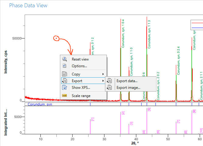
The data and pattern can be exported to different formats in several different ways. One way is to right-click on the pattern itself, and select Export from the menu.
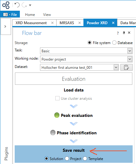
To save the data and analysis results, click the Save Result button. The pattern, peaks, peak search criteria, phase matches, and so on can be saved in individual files (Solution, as shown), or in multi-sample Projects, or as a Template. I think the template is the set of search and match criteria, the ones you used for this sample. It can be called back so the same criteria can be applied to any number of future samples, without clicking through all the steps. I’m not entirely sure of this, so look at the help files.
Advanced data analysis
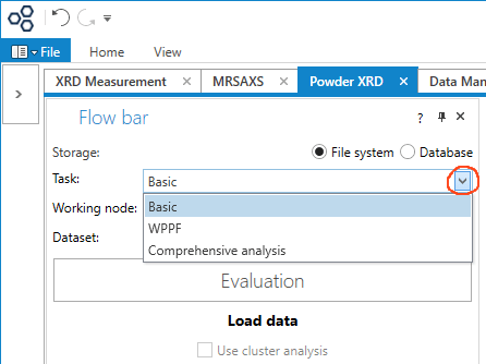
There are lots of other things you can do. Besides the Basic tasks described above, you can select WPPF, which includes Reitveld refinement, or Comprehensive analysis, which includes crystallite size, lattice strain, cell refinement, and crystallinity, including amorphous phases.

And lastly, if you look way down at the bottom of the Flow bar, you can see other analyses that you can do from within each Task type. See instructions.