SEM: Energy-Dispersive X-ray Analysis (EDS)

The SEM has a Bruker EDX system with a Peltier-cooled XFlash 6/30 silicon drift detector. The detector has an active area of 30 mm². It has an energy resolution of better than 123 eV at MnKα at count rates up to 60,000 cps (slightly lower resolution at count rates up to 275,000 cps). We have the software and a standard block for chemical analyses in standardized mode, though standardless analyses can be done too. In standardized mode, analyses are directly compared to standards of known chemical composition (minerals, glasses, metals, etc.), whereas in standardless mode the X-ray spectrum is fitted theoretically to derive a model composition. The results in standardless mode are surprisingly good, and can be used for many routine purposes like phase identification. Use standardized mode when accurate quantitative data are needed.

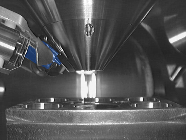The EDS detector is shown here, fully inserted into the vacuum chamber. It is behind the VP detector and in front of the SE detector. The EDS detector itself is a tiny chip inside the end of the detector tube, mounted on an insulated Peltier cooler. The detector can work with samples as close to the pole piece as 8.5 mm (nominal working distance), but higher count rates are available at a slightly lower position. In general, optimize the stage position for highest count rate, which should put the sample at the intersection point of the electron beam and the detector axis.

As the electron beam interacts with the sample, X-rays are produced. The X-ray continuum has energies ranging from the electron beam energy itself, on down to very low energies. The X-ray line spectrum is produced as electrons kick inner shell electrons out of sample atoms. As higher energy electrons in the atom lose energy to replace them, X-rays are emitted. The characteristic X-rays carry information about the presence and concentration of chemical elements in the samples. An X-ray hitting the detector produces several electron-hole pairs, the number approximately proportional to the incident X-ray energy. The charges are collected as a tiny current pulse. The tiny pulse is amplified and measured. Each measured pulse is then added to its proper energy bin (pulse size proportional to energy) to make a graph like that shown here. The X-axis is X-ray energy in keV, and the Y-axis is X-ray intensity. The red peaks correspond to characteristic X-ray lines emitted by elements in the sample. In this case the sample is apatite so we see strong lines for calcium (Ca), phosphorous (P), oxygen (O), and several smaller peaks. Note the Kα and Kβ lines are resolved for Ca but not for P. The size of these peaks, with the intensity and shape of the background on top of which the peaks sit, can be used to calculate the sample chemical composition. Chemical analyses are therefore one of the main results possible with this system.

Analyses can be exported as spreadsheet-readable tables, as spectra like that shown above, and also in a special format that can be accessed later for examination or reprocessing. This system has detection limits routinely near 0.1% (element weight), with element totals in standardless mode typically in the 100% ±10% range for common silicates. Element proportions, especially for elements sodium and heavier, are generally very good even when totals are not. Generally, the absolute uncertainty increases with decreasing atomic number and increasing interferences of the analyzed elements. In the example spectrum above, the error for oxygen is considerably more than the heavier elements phosphorous and calcium. Detection limits are typically much worse than wavelength-dispersive electron probe analyses. However, as the whole available X-ray spectrum is saved, elements not otherwise considered can be seen and processed in real-time or later. In contrast, with wavelength dispersive systems (WDS, e.g., electron probes) you must carefully choose the elements to analyze beforehand, and once done the analyses can’t tell you anything about other elements. The advantage of WDS is much better energy resolution (fewer and less serious interferences), much lower detection limits (higher peak/background ratios), and, at least compared to standardless EDS analyses, better accuracy especially for low concentration elements.

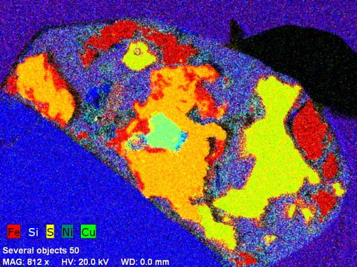
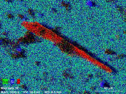
Another impressive capability of our system is fast X-ray mapping. The high count rate capability of our detector (up to 275,000 cps) and good energy resolution make it possible. Separate maps are made using narrow energy windows for elements of interest, and they can be color-coded and overlaid in real time (or later) to make a composite image. For example, this image is of a granite from Maine. Image data were collected using a beam current of 10 nA in about 15 minutes at an original resolution of 1024 x 768 pixels. Red is magnetite, light-brown is biotite, dark-brown streaks in biotite are chlorite, yellow-green is titanite, light-blue is apatite, dark-blue is zircon, gray is K-feldspar, dark-green is quartz, and medium-green (upper left) is plagioclase.

Plagioclase and K-feldspar in a granite from Maine. In the backscattered electron image the large gray crystal in the middle is intermediate plagioclase. It has a thin, darker-gray albite rim, which is the last plagioclase to crystallize. The lighter gray phase is K-feldspar, which has abundant dark-gray albite exsolution blobs. Some of the albite rim on plagioclase is exsolved from the K-feldspar. The light-gray phase is apatite, and white is magnetite and zircon. In the X-ray map (put cursor over the image) the zoning from Ca-rich core to Na-rich rim of the plagioclase is obvious. The K-feldspar is green, apatite yellow, and magnetite red. Note that the plagioclase also has K-feldspar inclusions.

This is a weathered sulfide crystal in a Norwegian eclogite, surrounded by silicates. In the backscattered electron image the weathered sulfide has a variety of irregular patches with different shades of gray. In the X-ray map (put cursor over the image), quartz and feldspar show up as blue and purple, respectively. Iron hydroxide is red, pyrite is orange, chalcopyrite is greenish-yellow, and a nickel sulfide is light-green. Initially the sulfide was probably a pyrrhotite solid solution.

This shows a comb-like structure growing in a hornblende amphibolite from the Adirondacks, NY. The dark-gray areas in the BSE image are plagioclase, with hornblende being the next lighter-gray, and orthopyroxene being the lightest gray. White specks are ilmenite. Dark-gray shreddy-looking things in the comb-like areas and elsewhere are apparently fine-grained muscovite, which may be related to the comb-forming reaction but more likely grew later. In the X-ray image (put cursor over the image), plagioclase is blue-green, hornblende is pink, orthopyroxene is red, muscovite is yellow-green, secondary calcite is dark-blue, and the small purple area at top center is clinopyroxene (calcic augite), which is not evident in the BSE image.

This is a slurry of a dissolved coprolite, dispersed on glass. The smooth background visible in the secondary electron image is glass. The long object is a bit of plant fossil. In the X-ray map (put cursor over the image) the plant fossil is highlighted by carbon X-rays shown in red. The glass background is blue-green from a combination of Na and Si X-rays. The dark specks are made of something else, though the dark-blue specks are probably quartz grains. The dark region to the right of the plant fossil is its own X-ray shadow, as X-rays from behind the fossil (relative to the detector) are absorbed.